Matrix reductions for eliminating spurious eigenvalues in the Chebyshev Tau method

The Cheyshev Tau method is a powerful tool for the numerical solution of eigenvalue boundary value problems. In particular, the so-called spectral convergence is faster than traditional FDM or FEM techniques by several orders of magnitude. However, when applied to problems of order $\geq 2$, spurious eigenvalues may appear (Dawkins et al.).

In this post we summarize a matrix factorization technique to modify the usual Tau method in order to eliminate the spurious values (Gardner et al.). The desired spectral convergence is preserved, which we verify with several test problems; notably one where the eigenvalue is located at the boundary. We also discuss using the Tau values to identify spurious or poor approximations to true eigenvalues.

The modified method is exceedingly useful for fixing a known issue with the Tau method. In fact, it can be shown to be equivalent to the modified Galerkin method where trial functions that obey boundary conditions are explicitely constructed. As this method requires less direct calculations, it seems to be the preferred choice.

The code for the post is written in Julia, and can be found in my spectral methods repository, which is to be developed into a package in the near future.

Chebyshev approximation

Some background on Chebyshev approxiation is required (Johnson). The Chebyshev polynomial of order $k$ is given by

$$\begin{align*} T_k(x) = \arccos(\cos(x)), \end{align*} \notag$$

for $x\in [-1,1]$, and satisfy the three-term recurrence relation $T_{k+1}(x) = 2x T_k (x) - T_{k-1}(x)$, with $T_0(x)=1$ and $T_1(x) = x$. The family $(T_k)_{k\geq 0}$ are an orthogonal basis with respect to the inner product

$$\langle f,g \rangle = \int_{-1}^{1} f(x)g(x)(1-x^2)^{-1/2}\text{dx}.$$

In particular we have $\langle T_i, T_j \rangle = c_i \pi\delta_{ij}/2$, where $c_i=1+\delta_{0i}$. Any smooth function $u$ and its derivatives can therefore be expanded as modal Chebyshev series:

$$\begin{align*} u(x) = \sum_{n=0}^\infty a_n T_n(x), && u^{(m)}(x) = \sum_{n=0}^\infty a_n^{(m)} T_n(x), && m=1,2,\ldots \end{align*}$$

Formulas for the derivative coefficients can be derived from the recursion relation $c_{n-1}a_{n-1}^{(m)} = 2na_n^{(m-1)} + a_{n+1}^{(m)}$, $n\geq 1$. In particular we have:

$$\begin{aligned} c_n a_n^{(1)} &= 2\sum_{\substack{p=n+1 \\ p + n\text{ odd}}}^\infty p a_p, \\ c_n a_n^{(2)} &= \sum_{\substack{p=n+2 \\ p + n\text{ even}}}^\infty p(p^2 -n^2)a_p, \\ c_n a_n^{(3)} &= \frac{1}{4}\sum_{\substack{p=n+3 \\ p + n\text{ odd}}}^\infty p(p^2(p^2-2) -2p^2n^2+(n^2-1))a_p, \\ c_n a_n^{(4)} &= \frac{1}{24}\sum_{\substack{p=n+4 \\ p + n\text{ even}}}^\infty p(p^2(p^2-4)^2 - 3p^4n^2 +3p^2n^4 - n^2(n^2-4)^2)a_p \end{aligned}$$

Formulas for higher derivatives can likewise be obtained. Another useful result gives the values of the $m$'th order derivative of a Chebyshev polynomial when evaluated at the end points:

$$T_n^{(m)}(\pm 1) = (\pm 1)^{n+m}\prod_{k=0}^{m-1}\frac{n^2-k^2}{2k+1}.$$

The above formulas are in terms of infinite sums, but in practice, we will work with truncated (finite) modal expansions.

Fourth order equations and the modified Tau method

We first consider a general fourth order equation of the form:

$$\begin{cases} L_1 v + L_2 u - s(v+L_3 u)=0 & x\in\Omega \\ v = L_4 u \end{cases}$$

where the $L_i$'s are (linear) second order differential operators, $u,v$ are the unknown eigenfunctions defined on a domain $\Omega$, and $s$ is the unknown eigenvalue. The problem may of course be formulated exclusively in terms of the eigenfunction $u$, but the factorization will be useful later. The Tau method involves truncating the Chebyshev expansions of $u$ and $v$ and taking the inner product to obtain a matrix system of equations. Unique to the Tau method is that the boudary conditions are imposed exactly, using (5). For our modified method, we write:

$$\begin{align*} u(x) \approx\sum_{n=0}^{N_{int}+N_{bou}-2} a_n T_n(x), && v(x) \approx \sum_{n=0}^{N_{int}+N_{bou}-2} b_n T_n(x), \end{align*}$$

where $N=N_{int}$ and $N_{bou}$ signifies the number of equations we obtain from the interior (governing) equations, and boundary conditions, respectively. Since we consider fourth order equations, we need exactly four boundary conditions, $N_{bou} = 4$, for the equation to be well-posed. Substituting the approximations into the governing equations and taking the inner product, we obtain a matrix system of the form:

$$\begin{aligned} &\bm{b} = Q\bm{a} \\ &B\bm{b} + A\bm{a} -s(\bm{b}+C\bm{a})=(\bm{0},\bm\tau)^T, \end{aligned}$$

where the $A,B,C,Q\in\mathbb R^{(N+3)^2}$ are the coefficient operators derived from $L_2,L_1,L_3,L_4$, respectively. The $\bm\tau=(\tau_1,\tau_2)$ coefficients are unknowns, and are used to indicate the rate of convergence. We now write $\bm{b}_1 = (b_0,\ldots,b_{N-2})^T$, $\bm{b}_2 = (b_{N-1},b_N)^T$, $\bm{y} = (b_{N+1},b_{N+2})$, and partition the matrices according to the following schematic:

$$\begin{aligned} &\left( \begin{array}{ccc|c} \\ & B_1 & & B_4 \\ \\ \hline & B_2 & & B_5 \\ \hline & B_3 & & B_6 \end{array} \right) \left(\begin{array}{c} \\ \bm{b}_1 \\ \\ \hline \bm{b}_2 \\ \hline \bm{y} \end{array}\right) + \left(\begin{array}{c} \\ A_1 \\ \\ \hline A_2 \\ \hline A_3 \end{array}\right) \left(\begin{array}{c} \\ \\ \bm{a} \\ \\ \\ \end{array}\right) \\ &\phantom{--------}-s\left(\begin{array}{c} \\ \bm{b}_1 \\ \\ \hline \bm{b}_2 \\ \hline \bm{y} \end{array}\right) -s\left(\begin{array}{c} \\ C_1 \\ \\ \hline C_2 \\ \hline C_3 \end{array}\right) \left(\begin{array}{c} \\ \\ \bm{a} \\ \\ \\ \end{array}\right) = \left(\begin{array}{c} \\ \\ \bm{0} \\ \\ \hline \bm\tau \end{array}\right) \\ \\ &\left(\begin{array}{c} \\ \bm{b}_1 \\ \\ \hline \bm{b}_2 \\ \hline \bm{y} \end{array}\right) = \left(\begin{array}{c} \\ Q_1 \\ \\ \hline Q_2 \\ \hline Q_3 \end{array}\right) \left(\begin{array}{c} \\ \\ \bm{a} \\ \\ \\ \end{array}\right) \end{aligned}$$

Writing $\bm{\hat{b}}$, we expand the block matrix equations:

$$\begin{aligned} & B_1\bm{\hat{b}} + B_4\bm{y} + A_1\bm{a} - s(\bm{b}_1+C_1\bm{a})=0, \\ & B_2\bm{\hat{b}} + B_5\bm{y} + A_2\bm{a} - s(\bm{b}_2+C_2\bm{a})=0. \end{aligned}$$

We can then isolate $\bm{y}$ in the second equation, requiring only a matrix inversion of $B_5\in\mathbb R^{2\times 2}$. With $\bm{b}_1=Q_1\bm{a}$ and $\bm{b}_2 = Q_2\bm{a}$ we get:

$$\begin{aligned} \bm{y} &=-B_5^{-1}\left[B_2\bm{b}+A_2\bm{a}-s(\bm{b}_2+C_2\bm{a}) \right] \\ &= -B_5^{-1}[B_2 Q + A_2 -s(Q_2 + C_2)]\bm{a} \end{aligned}$$

Substituting this into the first equation yields

$$\begin{aligned} [B_1Q-B_4 B_5^{-1}B_2Q + A_1 - B_4 B_5^{-1}A_2]\bm{a} = s[Q_1 + C_1 - B_4B_5^{-1}(Q_2 + C_2)]\bm{a}, \end{aligned}$$

which defines a generalized eigenvalue problem of the form $M\bm{a} = sN\bm{a}$, where $M,N\in\mathbb R^{(N-1)\times(N+3)}$. To obtain a square system, the boundary conditions may be viewed as a matrix equation $D\bm{a} =\bm{0}$ (with $D\in\mathbb R^{4\times (N+3)}$) that we concatenate to $M$. Writing $\bm{a_1}=(a_0,\ldots,a_N)^T$ amd $\bm{a_2} = (a_{N+1},a_{N+2})^T$ we further partition the complete system:

$$\begin{aligned} \left(\begin{array}{c|c} M_1 & M_2 \\ \hline D_1 & D_2 \end{array}\right) \end{aligned} \left(\begin{array}{c} \bm{a_1} \\ \hline \bm{a_2} \end{array}\right) = s \begin{aligned} \left(\begin{array}{c|c} N_1 & N_2 \\ \hline 0 & 0 \end{array}\right) \end{aligned}\bm{a}.$$

From the second block matrix equation we get $\bm{a_2} = -D_2^{-1} D_1\bm{a_1}$. Substituting into the first block matrix equation yields our final generalized eigenvalue problem:

$$(M_1 - M_2 D_2^{-1} D_1)\bm{a_1} = s(N_1 - N_2 D_2^{-1} D_1)\bm{a_1},$$

which can be solved with any appropriate eigenvalue solver. The final coefficients $\bm{a_2}$ are recovered from the previous equation.

The tau coefficients $\bm{\tau} = (\tau_1,\tau_2)^T$ are computed from the equation:

$$B_3\bm{\hat{b}} + B_6\bm{y} + A_3\bm{a} - s(\bm{y}+C_3\bm{a})=\bm{\tau},$$

Its magnitude is useful for identifying spurious eigenvalues, as well as indicating the degree of convergence of the modal coefficients $\bm{a}$. However, computing $\bm{\tau}$ also requires computing a normalized eigenvector corresponding to the eigenvalue, an increase in computational cost. Since only use the magnitude of the $\bm{\tau}$ coefficients are useful, we may simply consider the sum of its absolute values: if any one of the coefficients for a given eigenvalue have large magnitude, then that value is spurious or a poor approximation to a true eigenvalue.

Examples

We now illustrate the method on two different fourth order problems, with the notable difference being the location of the eigenvalue.

Consider first the fourth order boundary value problem with vanishing boundary conditions:

$$\begin{aligned} \begin{cases} u'''' + Ru'''-su''=0, & x\in (-1,1) \\ u(\pm 1) = u'(\pm 1) =0 \end{cases} \end{aligned}$$

where $R$ is a real parameter and $s$ is the eigenvalue. This is a standard example of an equation where the eigenvalue is located in the differential equation, and as such is present in all the interior modal equations. The modified method is implemented, and using a generalized Vandermonde matrix we can visualize the first few (normalized) eigenfunctions at the Chebyshev nodes:

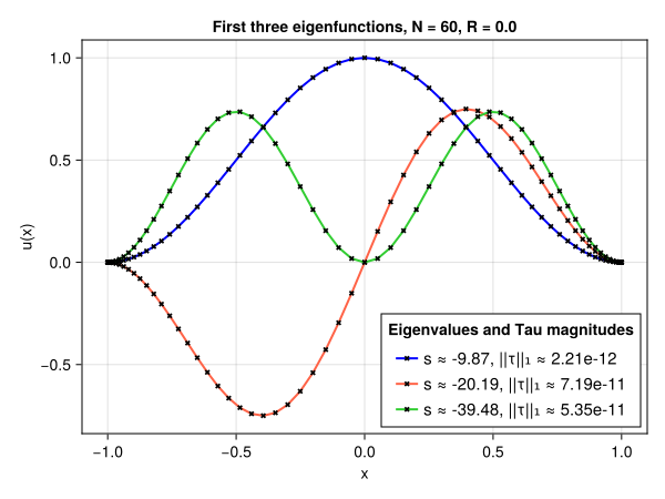
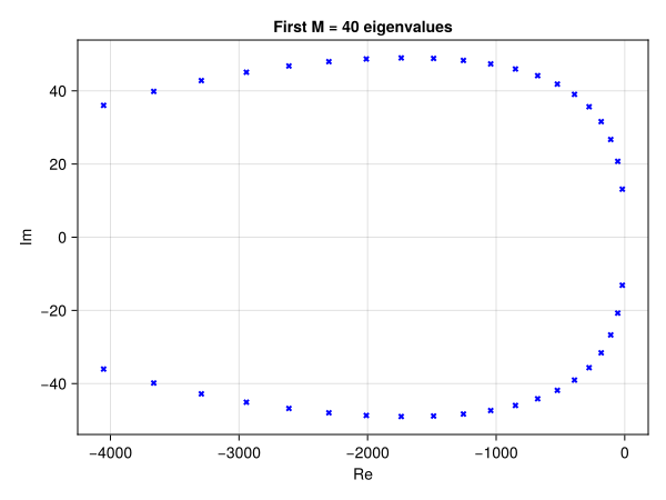
Observe that the boundary conditions are clearly obeyed. Furthermore, the associated Tau magnitudes for each eigenvalue are included, which indicate a good approximation to a true eigenvalue. Increasing the number of interior modes will increase the number of eigenvalues in the spectrum, but not all of them are good approximations to a true eigenvalue. However, no spurious eigenvalues appear at the start of the spectrum for any choice of $R$. For $R=0$ the differential operator is self-adjoint, so all eigenvalues are real, and in this case negative, numbers. In general, the spectrum will be a sequence of conjugate complex numbers with negative real part. This is seen in the following plot, for $R=5$:

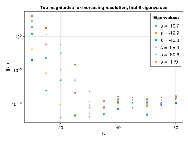
We observe from the Tau magnitudes in the following plot that the spectral convergence for the eigenvalues is obtained:

The same could most likely also be seen from computing the residual of the approximate eigenfunctions.

A defect of the method is that a very high number of modes will result in a ill-posed problem, and seemingly no true eigenvalues will appear in the spectrum. However, as the convergence plot shows, there is no reason for selecting such a high number of modes, unless one wishes to obtian a lot of eigenvalues. A possible remedy in this situation could be to use a spectral element method, partitioning the governing domain and therefore using several (low-mode) approximations to the eigenfunction. This is to be investigated further.

Consider now the following fourth order boundary value problem:

$$\begin{aligned} \begin{cases} u'''' -u'' + Ru=0, \qquad x\in (-1,1) \\ u(1) = u'(1) =0 \\ u'(-1) = u''(-1) + h\cdot u(-1)=0 \end{cases} \end{aligned}$$

where $R$ is once again a real parameter, and $h$ is the eigenvalue; it's location in a single boundary condition equation means that the analytic spectrum will be a singleton. However, our modified method will solve a very low-rank generalized eigenvalue problem. As such, eigenvalues of infinite magnitude are present in the spectrum, and will have to be removed by filtering. This suggests that solving the equation is ill-suited o be solved as a GEP, and some other method is preferred. It is possible that a constrained linear system can be solved, which would still leverage the effects of our modified method, but this is to be investigated further.

Nevertheless, the method can be implemented and the (normalized) eigenfunction can again be visualized at the Chebyshev nodes:

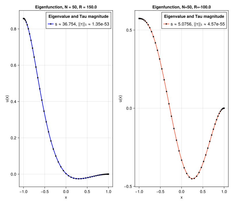
Observe that the rightmost boundary condition is clearly obeyed in both examples. Furthermore, the associated Tau magnitudes are seen to be extremely small, which could indicate a good approximation to the true eigenvalue. Further investigation of the Tau equation reveal only a small number of non-zero entries, which diminishes the information we can derive from them in this type of problem. To remedy this, one could compute the residual of the approximate eigenfunction, although we omit this here. We can however see a similar exponential convergence in the Tau magnitudes:

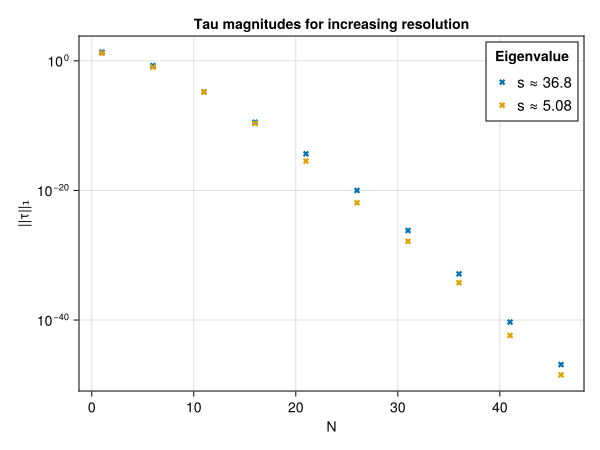
This plot indicates that the approximation converges (to something, but most likely the true solution to the equation).

Conclusion & future extensions

The modified Chebyshev Tau method was introduced and demonstrated to be a definite improvement of the standard Tau method when solving eigenvalue problems. So far, the implementations in the spectral methods repository is limited to homogenous problems with constant coefficients, but nonconstant coefficients are to be implemented in the near future. Nonlinear problems is a separate issue, that I am unsure how to tackle with this particular method. A first order linear approximation seems wasteful to pair with this modified method, since all the computation and precision gains would likely go to waste.

It is of great interest to implement a spectral element method, where this numerical scheme is to be used in each element. Generalizing to $2D$ and time-dependent problems is also an interesting direction to dedicate further effort. Overall this is a great first step in developing a suite for handling BVPs that appear in mathematical modelling.

References

• Gardner, Trogdon and Douglass, A Modified Tau Spectral Method That Eliminates Spurious Eigenvalues, 1988.

• Duane Johnson, Chebyshev Polynomials in the Spectral Tau Method and Applications to Eigenvalue Problems, 1996.

• Dawkins, Dunbar and Douglass, The Origin and Nature of Spurious Eigenvalues in the Spectral Tau Method, 1998.